A long, hands-on page about one formula: the runtime bound O(n + m + m·log(2 + m/(n+1)) + m⅓·(n·log(n+2))⅔) for C-HD, a directed single-source shortest-path algorithm that a September 2026 Vals AI writeup describes as designed by Claude agents and proved in Lean. Eleven sections take the bound apart term by term, set it against Dijkstra and the 2025–2026 Duan et al. bounds, and show where its formula comes out ahead with constants set to 1: a narrow band of sparse graphs, and on its own showcase profile only at astronomically large n.
How to use it
- 01 Anatomy: drag
vertices nandavg degree d. The bar splits the predicted operation count into its three terms, and the leaderboard compares every algorithm at that graph size. Hover a term in the formula to highlight it in the bar. - 02 Growth race: switch between
vary n (sparse → huge),vary densityandcertified profile (astronomical n)to see overhead over linear time as the graph grows. - 03 Exponent race: press
▶ play the history, or tap a year on the timeline, to add each bound from Bellman–Ford (1956–58) to C-HD. - 04 Zoom out: keep scrolling. Each frame adds more zeros on a doubly logarithmic axis, out to n ≈ 10^54,000, while a gauge tracks C-HD against Fibonacci-heap Dijkstra.
- 05 Who wins where: click a cell on the map to load that graph shape into section 01. In the 3D landscape below it, drag to orbit, scroll or pinch to zoom, and tick
apply certified rangeto drop the ground where C-HD falls back to Bellman–Ford. - 06–09 races:
▶ play,step,resetandnew graphdrive Dijkstra and band relaxation side by side; theband width Δslider moves between Dijkstra and Bellman–Ford behaviour. Section 07 steps through a model of C-HD withsize limit kandlevels. Section 09 offersSavannah · grid,Boston · tangleandParis · star; tap the map to move the start, and chooserace by roundsorrace by work. - 10 Live benchmark: pick an average degree and a maximum n, press
run sweep, thencopy CSVorcopy markdown. The 1M setting is slow.
How it works
Most of the charts evaluate textbook running-time formulas with every constant set to 1 and logs in base 2: Dijkstra with a binary heap, (n+m)·log n; with a Fibonacci heap, m + n·log n; a d-ary heap; Duan, Mao, Mao, Shu and Yin's 2025 m·log⅔ n; the 2026 Duan, Mao, Shu, Yin bound; Bellman–Ford, nm; and BFS as a floor. C-HD's formula is used only inside its certified range, m ≤ n·⌊⌊log₂n⌋¾⌋, and Bellman–Ford is charged outside it. The growth chart works in (log n, d) rather than n so it can run far past double-precision numbers. The exponent race sets the average degree to logα n and plots the remaining power of log n per vertex, which turns the "sorting barrier" into a flat line at 1.
The barrier comes from Dijkstra's algorithm settling vertices one at a time in exact distance order, which sorts them as a side effect. The newer algorithms avoid full ordering: bounded local searches from the frontier, a heap kept only over a thinned set of pivot vertices, and recursion in bounded batches. The page uses Δ-stepping, which relaxes every tentative distance in a band of width Δ together, as a simpler stand-in for that idea in the animated races.
Section 07 runs a scaled-down model of C-HD's FindPivots-HD step (bounded searches with a size limit, unexplored leaves counted against it, contact merges, permanent edge deletion) inside a Duan-et-al.-style bounded recursion, and checks each run against Dijkstra. It is not the Lean-verified program, which runs Bellman–Ford on any graph under 65,536 vertices. The street maps are OpenStreetMap snapshots contracted to intersections, with one-way streets honoured and trimmed to the largest strongly connected component. The benchmark builds random directed graphs in compressed sparse row form, runs binary-heap Dijkstra, Δ-stepping, queue-based Bellman–Ford and BFS, checks that the distances agree, and plots nanoseconds per edge. The 3D landscape is drawn with three.js.
Notes
Constants of 1 make the crossings a statement about growth rates, not stopwatch time, and the page notes that C-HD's real constants are large. The C-HD bound comes from a blog post with a machine-checked proof, not a peer-reviewed paper. Other sources cited on the page: arXiv 2504.17033, 2602.07868 and 2511.03007. Road data © OpenStreetMap contributors, ODbL.